Applications of Optimal Transport to Spatial Signal Processing Problems

In Defense of a Dissertation

David Gentile, 16 April 2026

Overview of the talk

Major goal is to introduce my two main projects:
- change point detection for time series analysis and,
- a barycentric coding model for measures on graphs
Unifying toolbox: the optimal transport (OT) problem and the geometry of probability distributions

Signal Processing

A Rich Tradition in Applied Mathematics

A signal is just a function. Often it’s a function in time, but for today we’ll actually be interested in functions of space as well.
Three tasks today: pattern identification, analysis of a signal and synthesis of a signal
Pattern Identification: Looking for common themes in the data
Analysis: understanding a signal in terms of some essential set of components
Synthesis: building a new signal out of some essential set of components

Signal Processing

What kind of signals do we care about?

Today, we’ll restrict to a very specific kind of signal: probability measures.
A probability measure is a non-negative function on some domain \(\Omega\) that sums (integrates) to \(1\).
The set of all probability measures on a given domain I’ll denote by \(\P(\Omega)\)
If \(\Omega = \R^d\), we may also make reference to the space of finite variance and absolutely continuous measures \(\P_{2,ac}(\Omega)\)
If we’re willing to conceptualize the domain \(\Omega\) as a physical space, we can also think of a probability measure as being a “pile of sand with unit mass”, which we might want to transport around, depending on our needs

Signal Processing

What do I mean by “spatial” signal processing?

By “spatial” signal processing, I mean specifically any signal processing problem where the underlying geometry of the domain plays an important role
Major point: because these problems are informed by the geometry of the underlying domain, we want some tool that encodes that information and makes use of it
Enter…

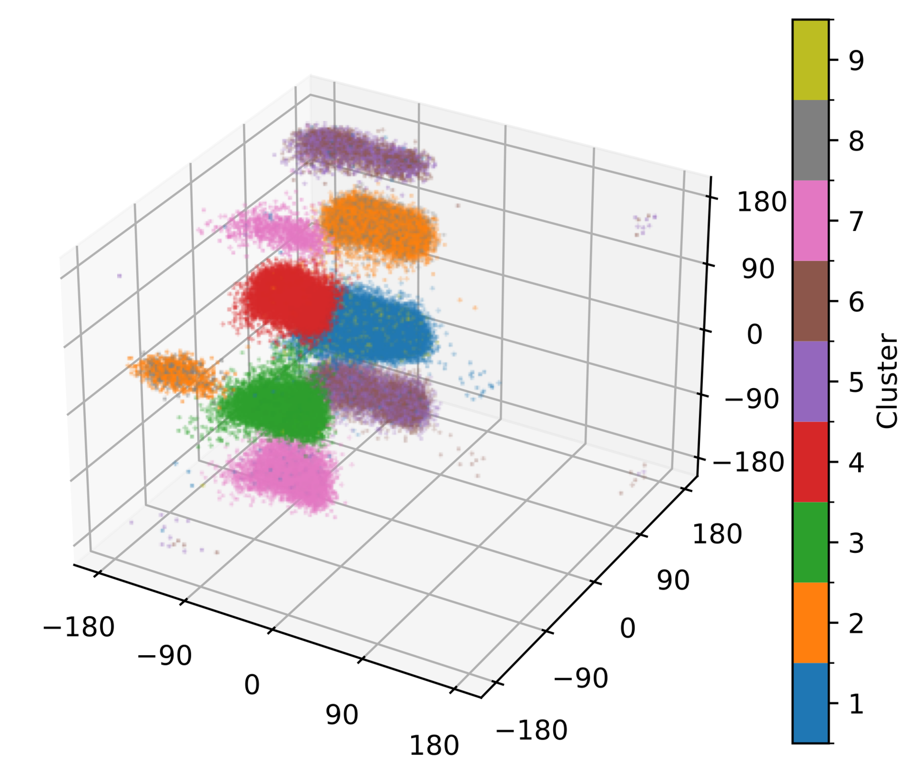
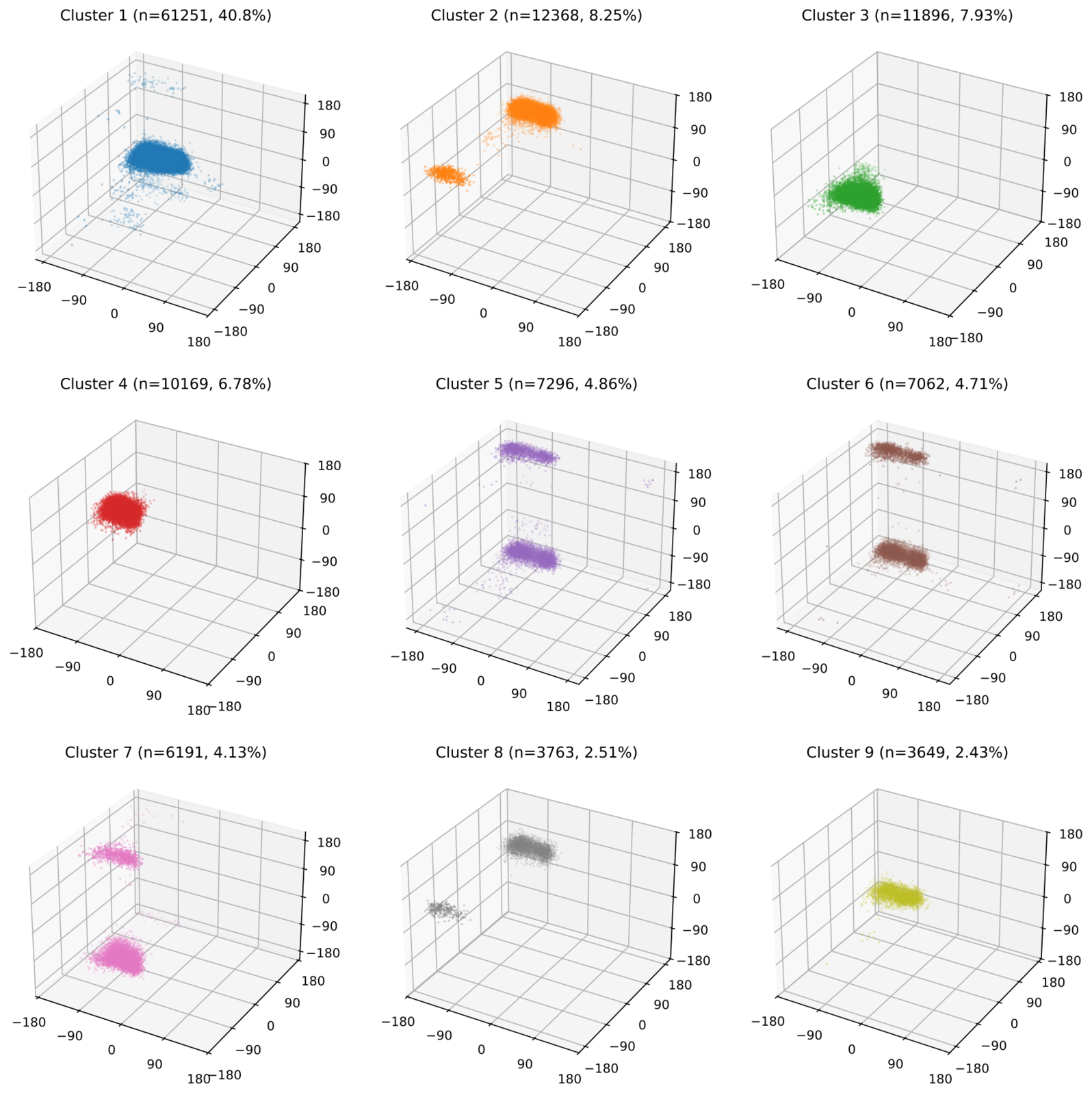
3D scatter of a valine dipeptide trajectory in dihedral-angle space, coloured by cluster

Optimal Transport:

A Tool for Comparing Probability Distributions

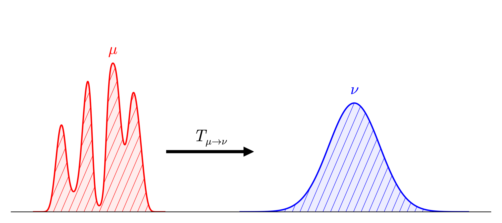
A multimodal density mu transported onto a unimodal density nu by a map T

Background on Optimal Transport

Kantorovich Problem, Wasserstein Geometry

Let \(\mu, \nu \in \P(\Omega)\), \(c : \Omega \times \Omega \to \R^+\). Then the optimal transport cost between \(\mu\) and \(\nu\) is given by the minimal value of the Kantorovich problem:
\[ \OT(\mu,\nu) = \inf\left\{ \int_{\Omega\times\Omega} c(x,y)\, d\gamma(x,y) : \gamma \in \Pi(\mu,\nu) \right\} \]
Remarkable fact: if \(\Omega = \R^d\), \(c(x,y) = \|x-y\|^2\), and we limit ourselves to probability measures of finite variance, then the square root of the optimal transport cost is a metric on \(\P_{2,ac}(\Omega)\), denoted by \(W_2\),
\[ W_2^2(\mu,\nu) = \inf\left\{ \int_{\Omega\times\Omega} \|x-y\|^2\, d\gamma(x,y) : \gamma \in \Pi(\mu,\nu) \right\}. \]

Background on Optimal Transport

How does transport encode information about the underlying domain?

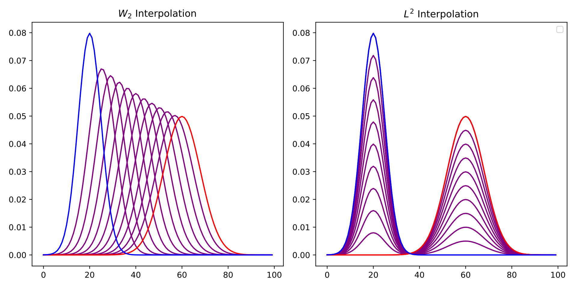
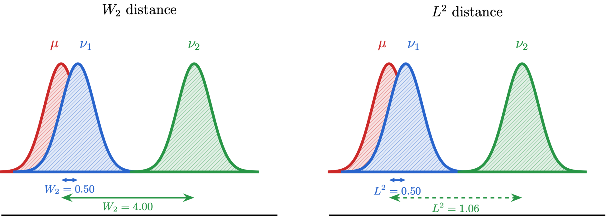
Interpolation between two densities in the W2 geometry (mass slides across) and the L2 geometry (mass fades in and out)

Schematic: W2 interpolation moves mass horizontally, L2 interpolation moves it vertically

The \(W_2\) distance between two distributions tells us how expensive it is to move one to the other “physically”
This contrasts with, e.g., the \(L^2\) difference between the densities of two distributions, where mass “teleports”

Background on Optimal Transport

Metric Derivative in the Wasserstein Geometry

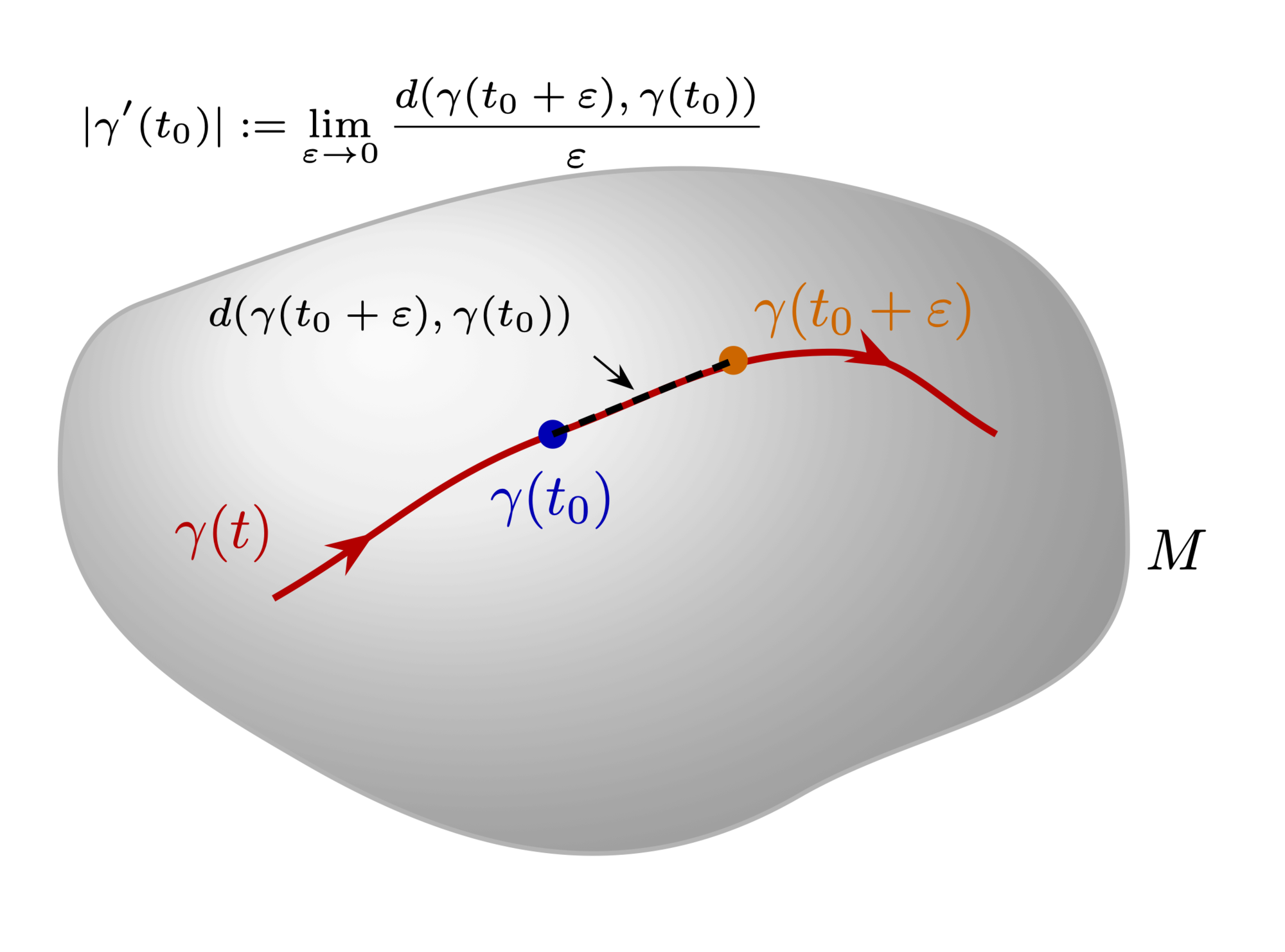
A curve gamma(t) on a manifold with the metric derivative defined as the limit of d(gamma(t0 + eps), gamma(t0)) / eps

A tool we’ll use for the CPD approach is the metric derivative, which we will try to estimate based on data
Intuition: difference quotient of a curve in space measuring its instantaneous speed (no direction information)
We will use this to measure the rate at which a local ensemble of data points is evolving in the space of probability distributions!

Application: A Transport Motivated Approach to Time Series Clustering

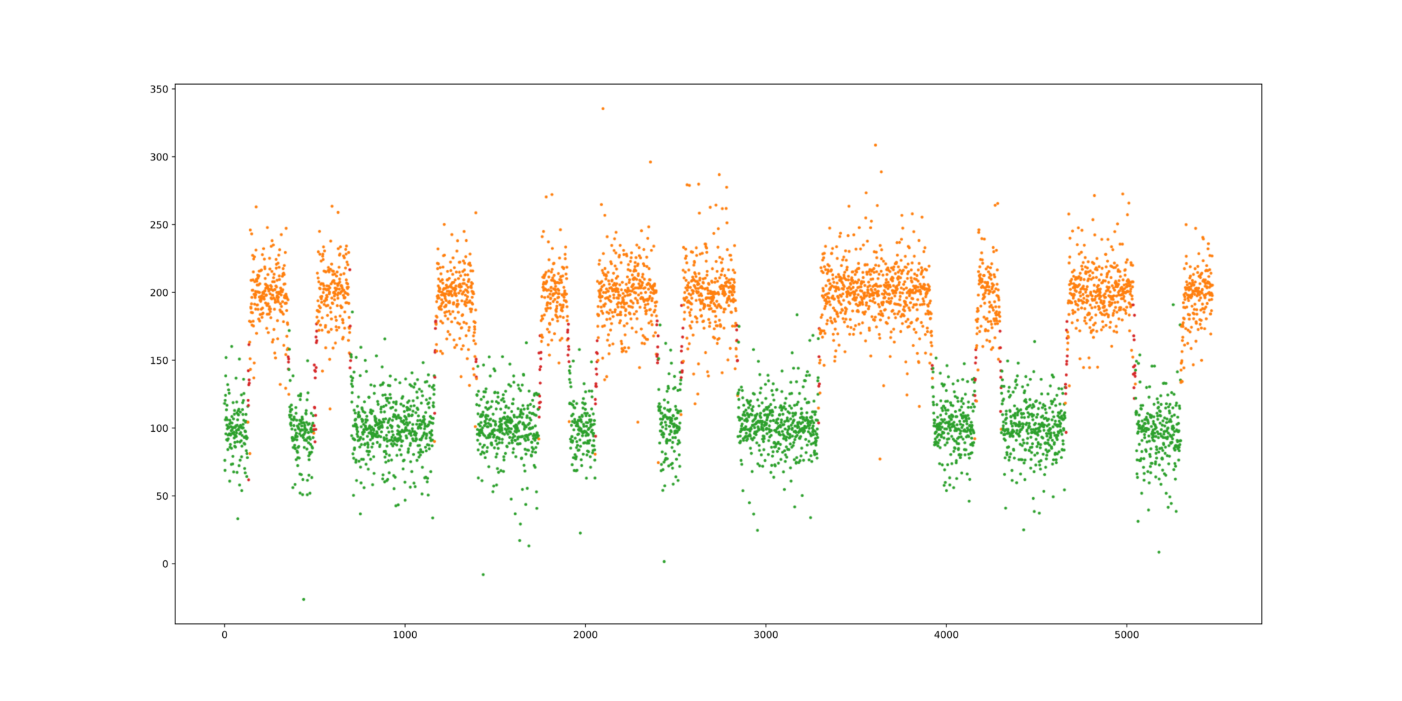
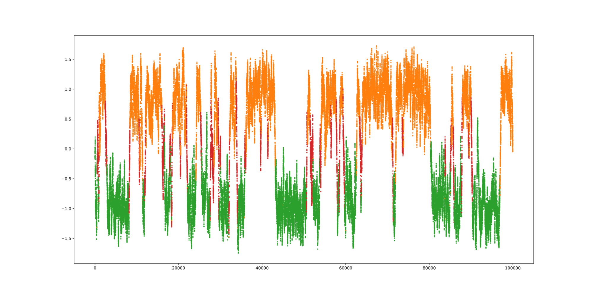
A time series whose samples are coloured by the cluster they were assigned to

Problem: Detecting Change Points in a Time Series

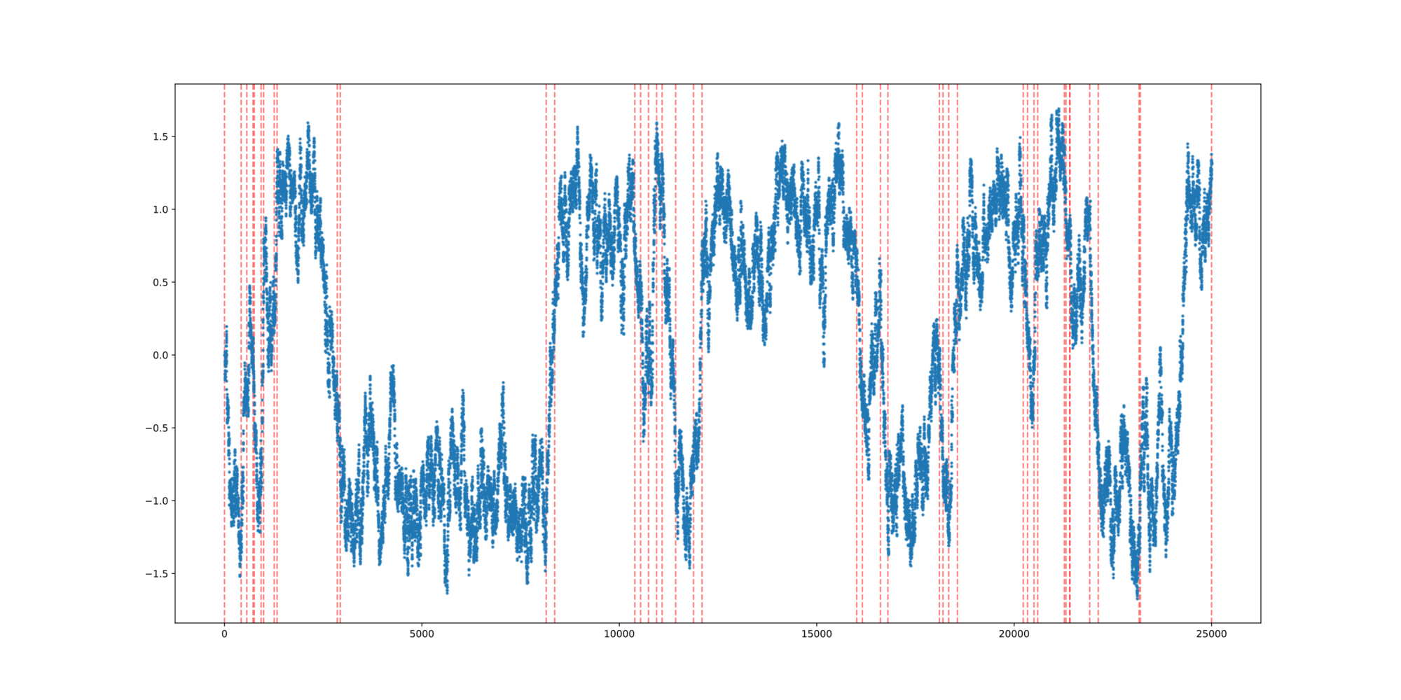
Given a realization of a stochastic process \(\{X_t\}_{t=1}^{T}\), we want to detect when significant changes to the law of the process occur
Main idea: better to look at many samples simultaneously to get a better sense of the overall state of the process and robustly identify patterns and structures in the observed data

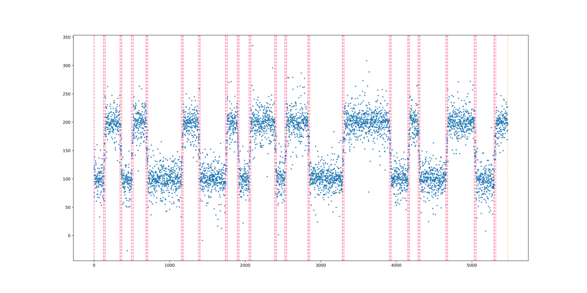
A noisy time series with vertical lines marking the times at which its distribution changes

Detecting Changes with the Optimal Transport Cost

Key Idea: Changes happen when neighboring distributions differ in \(W_2\)

We use a sliding window approach to look for CPs
At each step we approximate the metric \(W_2\) derivative between neighboring batches of \(w\) samples
Then a quantile-based cutoff is applied to identify CP candidates, which are further culled by identifying inflection points of the metric derivative data in contiguous segments

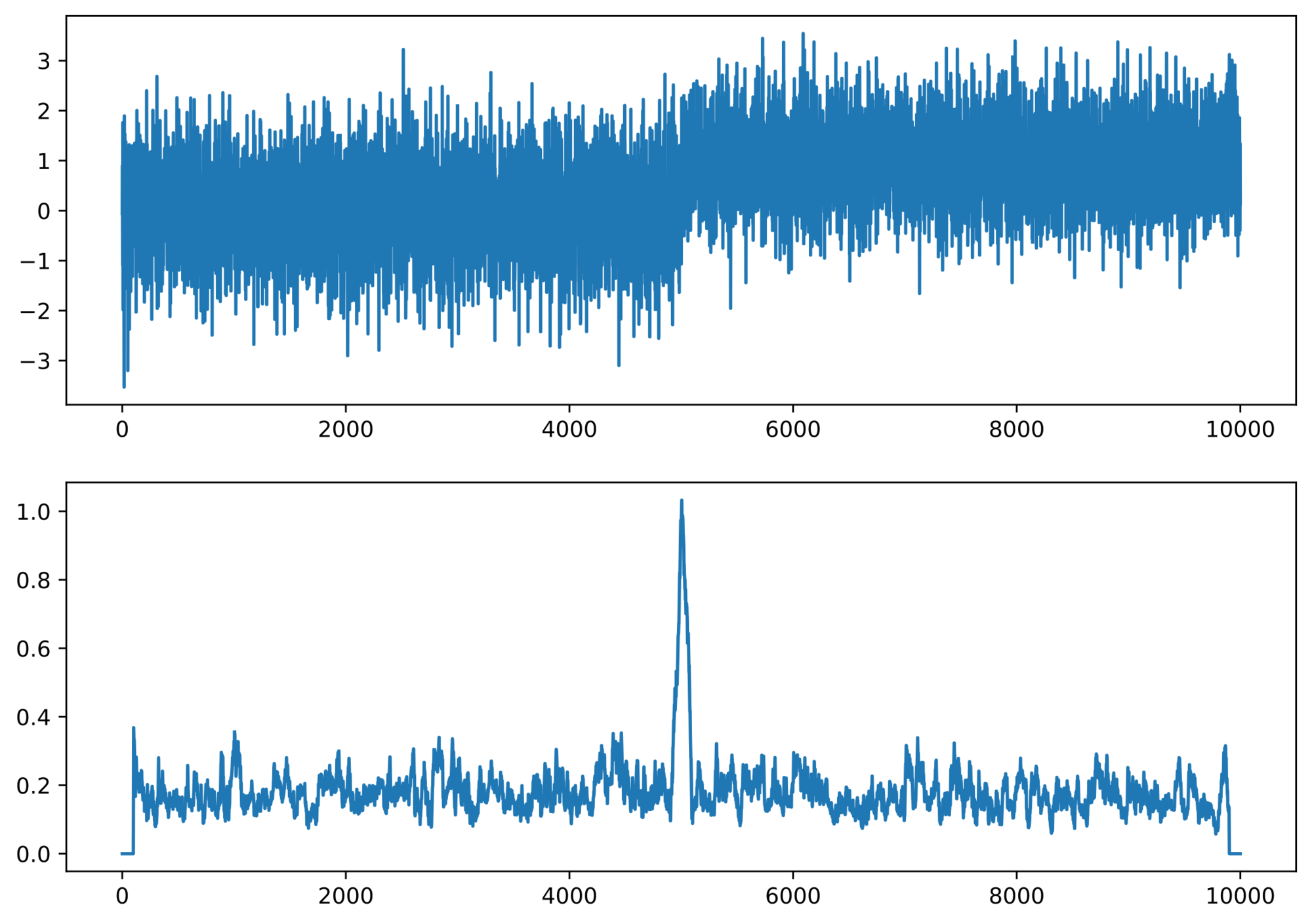
Top: a time series. Bottom: its estimated W2 metric derivative, which spikes at the change point

Clustering Segments based on Change Points

Key Idea: Quantify Segment Similarity with \(W_2\)

We compute pairwise segment similarity by measuring their distance in \(W_2\)
Then we use a “classical” clustering algorithm (ADPC) that analyzes the pairwise distance matrix
For multidimensional data, we carry this procedure out on each component of the data and then glue the resulting labels together

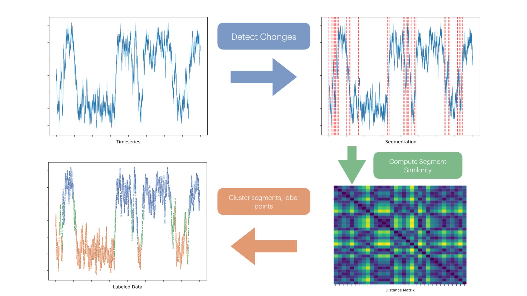
Pipeline: time series, detected change points, pairwise W2 distance heatmap between segments, clustered time series

Numerical Experiment

Clustering a particle trajectory driven by Langevin dynamics

Trajectory of a particle in a double-well potential

The same trajectory coloured by cluster label

Example: trajectory of a particle in a double-well potential
Clustering reveals both wells and a transition state between the two meta-stable ones

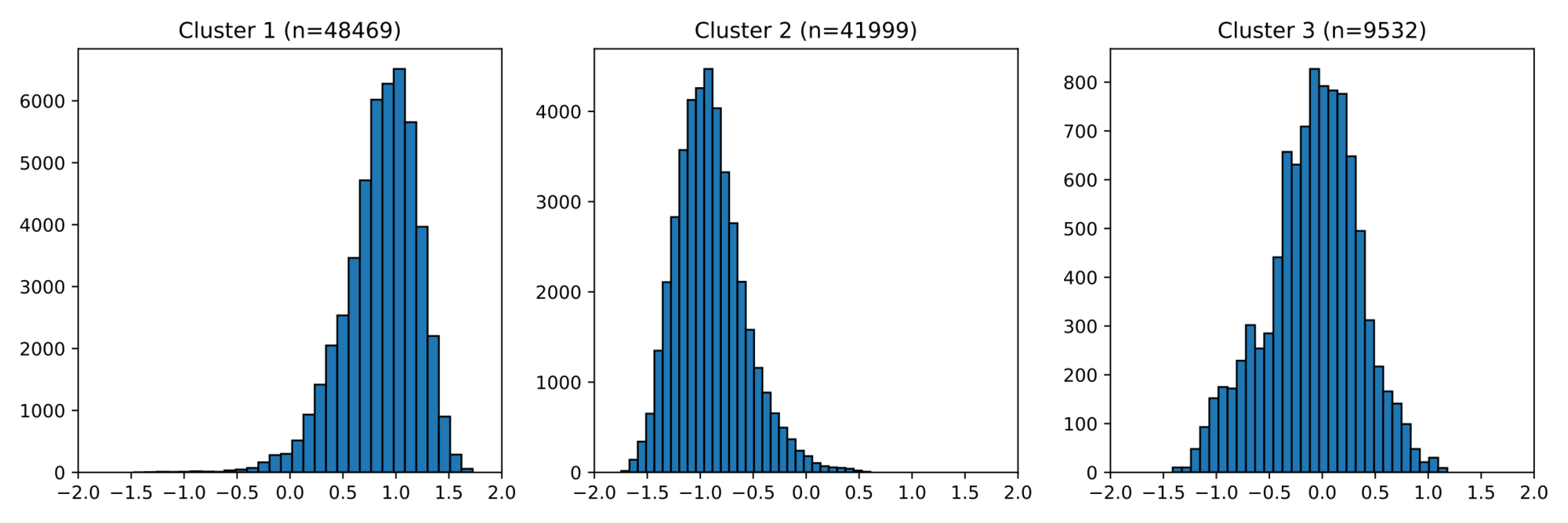
Histograms of the three clusters' empirical distributions

Numerical Experiment

Clustering A Valine Dipeptide Trajectory

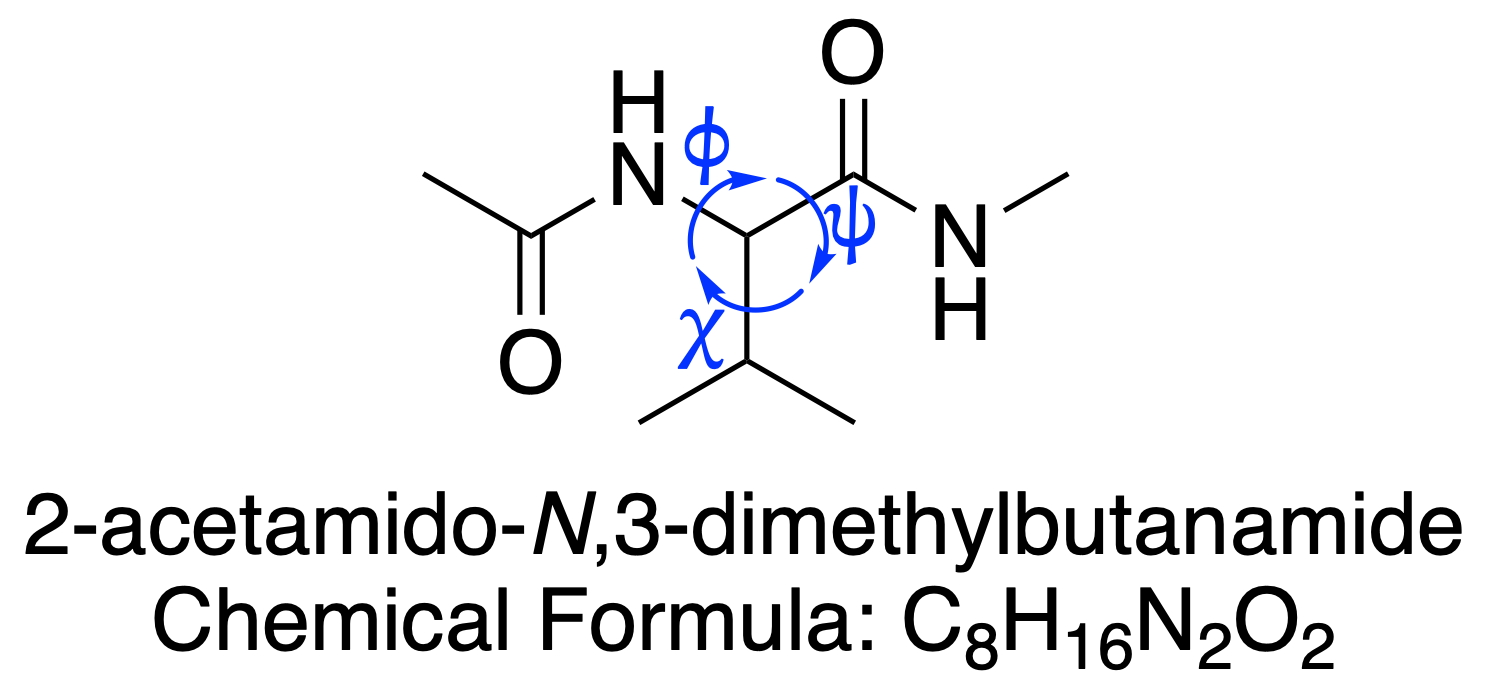
Chemical structure of valine dipeptide (2-acetamido-N,3-dimethylbutanamide)

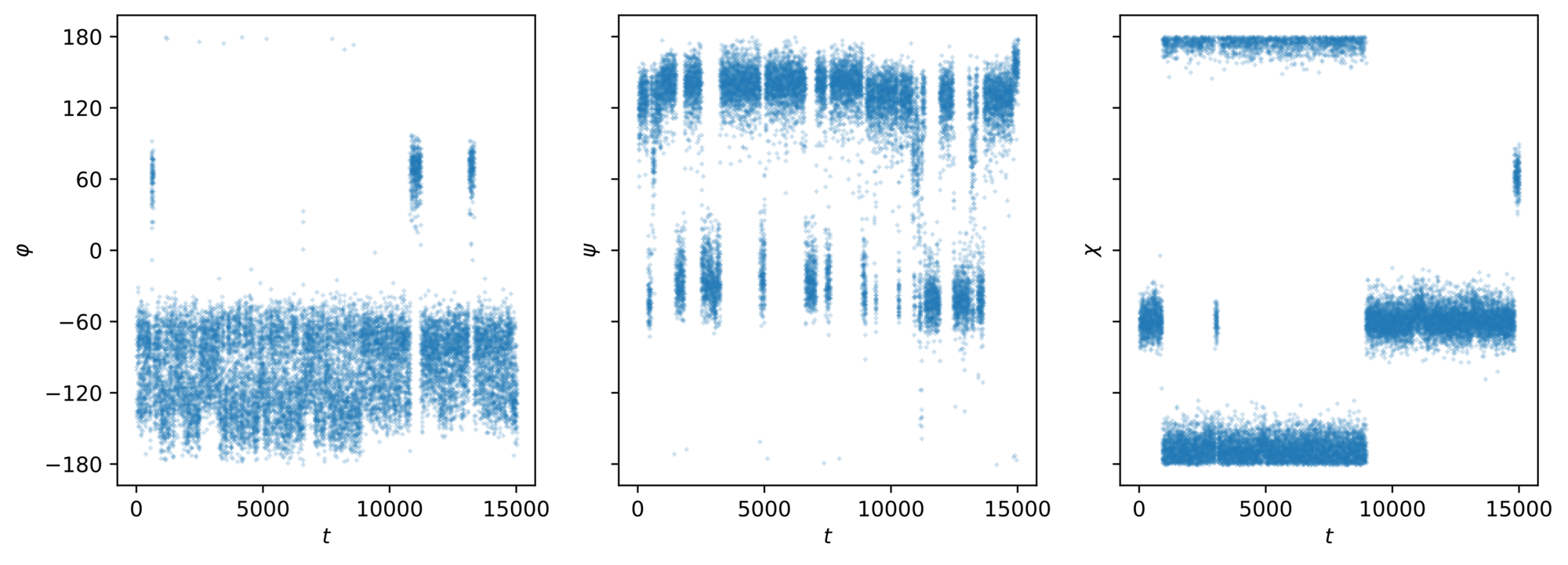
The three dihedral-angle time series phi, psi and chi of a valine dipeptide trajectory

Numerical Experiment

Clustering A Valine Dipeptide Trajectory

All clusters of the valine dipeptide trajectory in dihedral-angle space

Takeaways

For Applications of Optimal Transport to CPD

We applied optimal transport to identify from data patterns in the phase space of an observed stochastic process
Did this by concocting an algorithm that identifies a segmentation of a given time series in a non-parametric way (i.e., no assumptions on the underlying distribution)
We cluster the segments in \(W_2\) space and get natural looking clusters for the trajectory in its phase space

A Barycentric Coding Model for Measures on Graphs

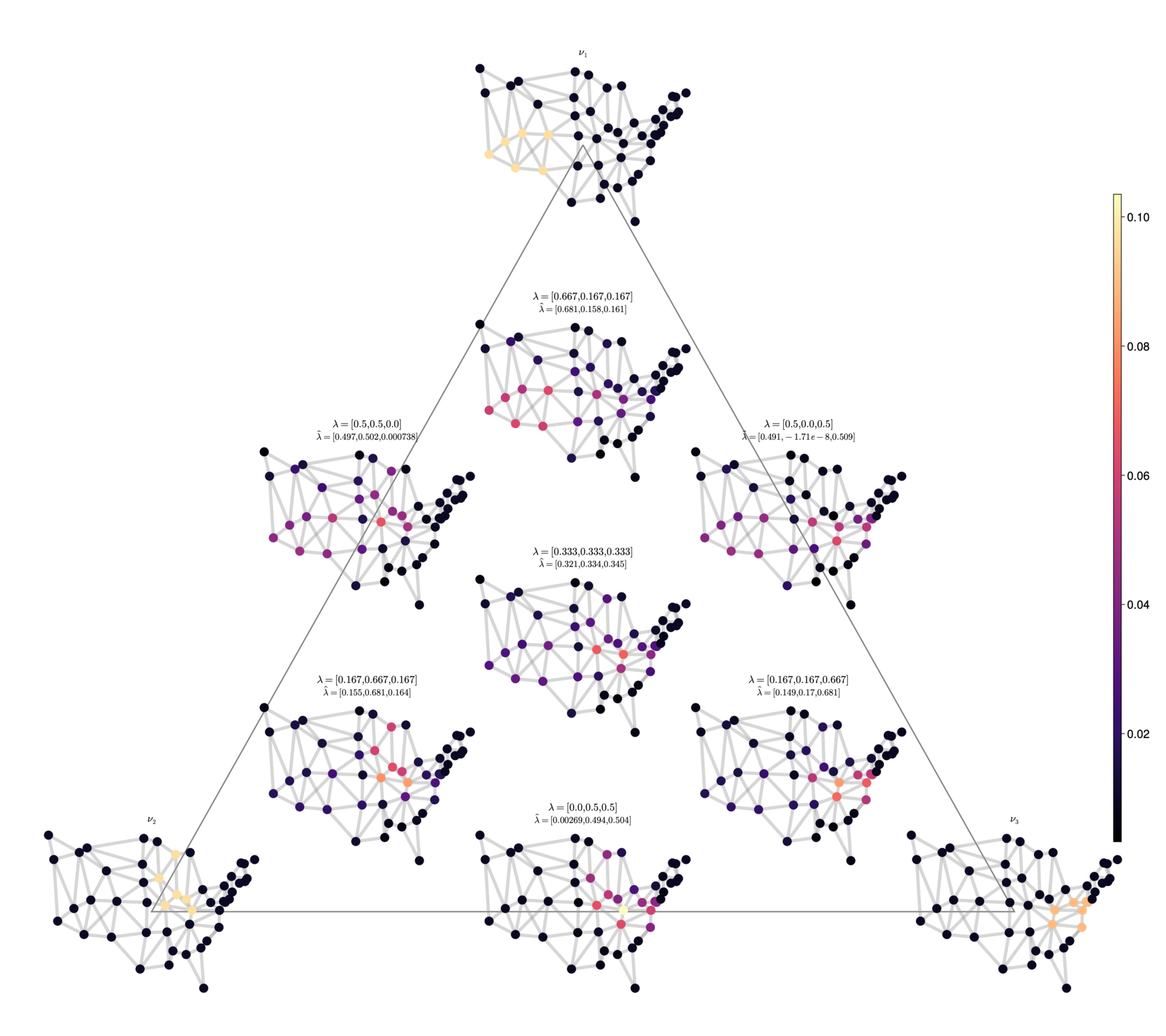
A triangle of measures on the US states graph: reference measures at the vertices, barycenters inside

Structure for this part of the talk

Switching gears

Motivate the barycentric coding model (BCM) in general
Explain why transport on graphs requires some extra machinery
Show how we leverage that machinery to implement the BCM
Highlight some visual results from our numerical experiments
Conclude with musings about future directions this project might take

What the heck is a barycentric coding model?

And why is it for “measures”?

A barycentric coding model is a way of using a set of essential components (“dictionary atoms”) \(\Refs = \{\nu_i\}_{i=1}^{p}\) to construct and analyze a broad family of measures in terms of simplicial weights \(\lambda \in \Delta^{p-1}\)
\[ \Delta^{p-1} = \left\{ (\lambda_1, \dots, \lambda_p) : \textstyle\sum \lambda_i = 1,\ \lambda_i \ge 0 \right\} \]
A barycenter of measures is a weighted center of mass in the transport geometry.
Two jobs we want to do numerically:
- Synthesis: ID the weighted center of mass \(\nu_\lambda\), given \(\lambda \in \Delta^{p-1}\) and \(\Refs = \{\nu_i\}_{i=1}^{p}\)
- Analysis: ID the weights \(\lambda \in \Delta^{p-1}\) for given \(\nu_0\), \(\Refs = \{\nu_i\}_{i=1}^{p}\)

Example BCM

Vertices of the triangle correspond to dictionary atoms
Points inside the triangle are syntheses of the measures on the vertices
Measures are annotated with their “true” coordinates and the coordinates recovered by our analysis algorithm.

A triangle of measures on the US states graph, annotated with true and recovered barycentric coordinates

Definitions

Graphs & Markov Transition Kernels

A graph is an example of a discrete metric space.
A graph is defined by vertices and edges, and we typically write something like \(X = (V, E)\), sometimes with an associated (symmetric) weight matrix \(\omega : E \to \R^+\) (if unspecified, \(\omega \equiv 1\ \forall (x,y) \in E\))
We will assume our graphs are simple, and can be represented by a Markov transition kernel \(Q\) with unique steady state distribution \(\pi\)

\[ \pi(x) = \frac{\deg_\omega(x)}{\sum_{y \in V} \deg_\omega(y)}; \qquad Q(x,y) = \begin{cases} \dfrac{\omega(x,y)}{\deg_\omega(x)} & (x,y) \in E \\[0.6em] 0 & \text{else.} \end{cases} \]

Definitions

Functions, vectors, probability measures on graphs

A function \(\varphi\) on \(X\) is a function on its vertices and therefore a vector in \(\R^{|V|}\)
A vector field \(\Phi\) on \(X\) is a function on its edges, and therefore a vector in \(\R^{|V| \times |V|}\)
For technical reasons, we’ll consider probability measures with respect to the steady vector \(\pi\), i.e.,

\[ \P(X) = \left\{ \nu \in \R_+^{|V|} : \sum_{x \in X} \nu(x)\pi(x) = 1 \right\} \]

Barycenters, Classic Edition

Motivation: Convex combinations in \(\R^d\)

In \(\R^d\), given points \(\{x_i\}_{i=1}^{p}\) and weights \(\lambda = (\lambda_1, \dots, \lambda_p) : \sum \lambda_i = 1\), it’s easy to combine the points:
\[ x = \sum_{i=1}^{p} \lambda_i x_i \]
But lots of spaces lack the linear structure that enables this straightforward combination
Idea: observe that \(x\) solves a certain optimization problem:
\[ x = \operatorname*{arg\,min} \sum \frac{\lambda_i}{2} \|x - x_i\|^2 \]

Barycenters Classic Edition

Motivation: Barycenters of Measures in the \(W_2\) geometry

To define a weighted average \(\nu_\lambda\) of measures \(\Refs = \{\nu_i\}_{i=1}^{p} \subset \P_{2,ac}(\Omega)\) for given weights \(\lambda \in \Delta^{p-1}\), we look for minimizers of sums of squared distances, solving:
\[ \inf\left\{ J[\nu] = \sum_{i=1}^{p} \frac{\lambda_i}{2} W_2^2(\nu, \nu_i) \right\} \]
We’ll sometimes refer to \(J\) as the variance functional. It’s a major theorem that in the Euclidean setting, minimizers of \(J\) exist and are unique under appropriate technical conditions, see Agueh & Carlier (2011) for details.

Agueh, Carlier. “Barycenters in the Wasserstein space.” SIAM Journal on Mathematical Analysis 43.2 (2011): 904–924

Why is this even a problem?

Degeneracy of the Classical Transport Geometry when \(|\Omega| < \infty\)

Consider the case \(X_2 = \{a, b\}\), then every measure \(\nu \in \P(X_2)\) looks like \(\nu = \nu_\alpha = (1-\alpha,\, 1+\alpha),\ \alpha \in [-1, 1]\)
Exercise to the reader: use a little linear algebra to characterize every coupling for a fixed pair of measures \(\nu_\alpha, \nu_\beta \in \P(X_2)\) and solve the K.P. explicitly
Conclude that \(\left(\P(X_2), W_2\right) \simeq \left([0,1], \sqrt{|x-y|}\right)\)
Further conclude that if \(\nu(t) : [0,1] \to \P(X_2)\) is a geodesic curve then it is constant! So you can’t even define a barycenter of two measures on a two point graph. Sad fact of life.

More Background on Optimal Transport

Benamou-Brenier Formula

Cool transport fact: \(W_2\) can be interpreted as arising from a certain Riemannian structure on an “infinite dimensional manifold”, via the Benamou-Brenier formula (see Benamou & Brenier (2000) for details)
\[ W_2^2(\rho_0, \rho_1) = \inf\left\{ \A(\rho(x,t), V(x,t)) = \int_0^1 \|V(t,x)\|^2_{L^2(\rho(t,x))}\, dt \right\} \]
The infimum is taken over pairs \(\rho : [0,1] \times \R^d \to \R\), \(V : [0,1] \times \R^d \to \R^d\) which satisfy the continuity equation with temporal boundary conditions:
\[ \frac{\partial \rho}{\partial t} + \nabla \cdot (\rho V) = 0; \qquad \rho(0, \cdot) = \rho_0,\ \rho(1, \cdot) = \rho_1 \]

Benamou, Jean-David, and Yann Brenier. “A computational fluid mechanics solution to the Monge-Kantorovich mass transfer problem.” Numerische Mathematik 84.3 (2000): 375–393.

How to Put a Continuity Equation on a Graph

Calculus on Graphs

First, we need to define some differential operators in the graph setting:
The gradient of a function \(\varphi\) is a vector field \(\gradX \varphi\) defined by the expression
\[ \gradX \varphi(x,y) = \varphi(x) - \varphi(y) \]
The divergence of a vector field \(\Phi\) is a function \(\divX \Phi\) defined by the expression
\[ \divX \Phi(x) = \frac{1}{2} \sum_{y \in X} Q(x,y)\left(\Phi(y,x) - \Phi(x,y)\right) \]

Continuity Equations on Graphs Cont’d

More Calculus on Graphs

Finally we can combine the gradient and divergence operators to obtain a graph Laplacian. The graph Laplacian of a function \(\varphi\) is another function \(\Delta_X \varphi\) defined by the expression
\[ \begin{aligned} \Delta_X \varphi(x) &= \sum_{y \in X} Q(x,y)\left(\varphi(y) - \varphi(x)\right), \\ &= (Q - D)\varphi, \end{aligned} \]
where \(D = \operatorname{diag}\left( \sum_{y \in X} Q(x,y) \right)\)

Continuity Equations on Graphs

The admissible mean

Notice: need to make sense of the product \(\rho V\) in the CE
\[ \frac{\partial \rho}{\partial t} + \nabla \cdot (\rho V) = 0 \]
An admissible mean is a function \(\theta : \R^+ \times \R^+ \to \R^+\); it must be concave, lower semi-continuous, 1-homogeneous, symmetric, and \(C^2\) on \((0,\infty)^2\).
Examples:
\[ \theta_{\log}(s,t) = \frac{s-t}{\log(s) - \log(t)}; \qquad \theta_{geo}(s,t) = \sqrt{st} \]
For \(\rho \in \P(X)\), define \(\theta(\rho)(x,y) = \theta(\rho(x), \rho(y))\); now \(\theta\) turns functions into vector fields

Continuity Equations on Graphs, Cont’d

Finally: we write down a continuity equation

We now have the language to express a discrete continuity equation

\[ \CE(\rho_A, \rho_B) := \left\{ (\rho, m) : \frac{\partial \rho}{\partial t} + \divX(\theta(\rho) \odot m) = 0,\ \rho(0,\cdot) = \rho_A,\ \rho(1,\cdot) = \rho_B \right\} \]

\[ \A(\rho, m) := \frac{1}{2} \int_0^1 \sum_{i,j \in X} \frac{m(t,i,j)^2}{\theta(\rho(t,i), \rho(t,j))}\, Q(i,j)\pi(i)\, dt. \]

\[ \W(\rho_A, \rho_B) := \inf\left\{ \sqrt{\A(\rho, m)} : (\rho, m) \in \CE(\rho_A, \rho_B) \right\}. \]

Maas, Jan. “Gradient flows of the entropy for finite Markov chains.” Journal of Functional Analysis 261.8 (2011): 2250–2292.

The \(\W\) Geometry

Getting back towards barycenters

Recall that the variance functional is expressed directly in terms of a metric!
\[ J[\nu] = \sum_{i=1}^{p} \frac{\lambda_i}{2} \W^2(\nu_i, \nu) \]
We want to minimize it, and to do that we’ll use one of the oldest tricks in the book: gradient descent
Main idea: look for the direction in which \(J\) is decreasing most rapidly, and take a “small step” in that direction
Two problems now: 1) how do I know what direction to walk in and 2), how do I walk in it?

The \(\W\) Geometry, Cont’d

Riemannian Geometry Objects: Tangent Space & Metric Tensor

We’ll need to understand two things about the Riemannian geometry of \((\P(X), \W)\): the metric tensor, and the exponential mapping
First, we need to say what the tangent space is, and how we can compute the inner product of two vectors at a point. This turns out to be relatively easy!

\[ T_\nu \P(X) = \left\{ \nabla\varphi \in \R^{|V| \times |V|} : \varphi \in \R^{|V|} \right\}, \]

\[ \langle \nabla\varphi, \nabla\psi \rangle_\nu = \frac{1}{2} \sum_{x,y \in V} \theta(\nu(x), \nu(y))\, \nabla\varphi(x,y)\, \nabla\psi(x,y). \]

The \(\W\) Geometry, Cont’d

Riemannian Geometry Objects: Exponential Mapping and Inverse

Now on any generic Riemannian manifold, one can consider the exponential mapping and its inverse, which relates the local geometry of the manifold to its tangent space
\[ \exp_\nu : U \subset T_\nu \P(X) \to \P(X), \]
If \(\gamma_{\nu,m} : [0,1] \to \P(X)\) is a geodesic curve with \(\gamma(0) = \nu,\ \gamma'(0) = m\), then
\[ \exp_\nu(m) = \gamma_{\nu,m}(1), \]
and
\[ \exp_\nu^{-1}(\gamma_{\nu,m}(1)) = m. \]

Synthesis Plan: Intrinsic Gradient Descent

When in Non-Euclidean spaces, do as the Non-Euclidean Optimizers Do

Classic way to optimize a function: gradient descent
\[ x_{k+1} = x_k - t_k \nabla F(x_k) \]
Compute the gradient, walk in the direction of steepest descent, eventually find a minimum where \(\nabla F(x_\infty) = 0\)
We’ll do something similar here, but to keep ourselves on the set \(\P(X)\), we will use the intrinsic gradient associated to a certain Riemannian structure

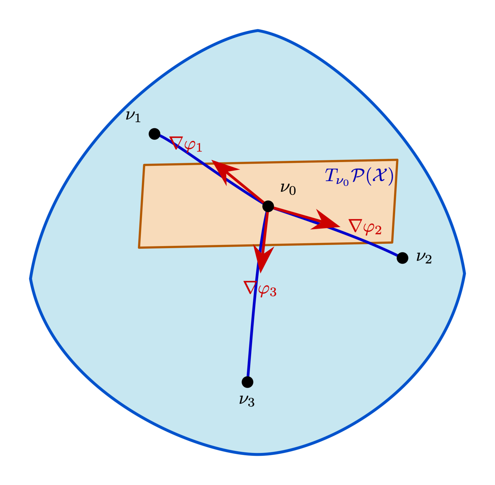
A curved manifold with a tangent plane at the current iterate; the descent direction lives in the tangent plane and is mapped back to the manifold

Analysis Plan: Inverting The Exponential Map

Take it to the Tangent Space

In order to analyze measures with respect to a family of references \(\Refs\), we leverage a theorem due to Werenski et al.

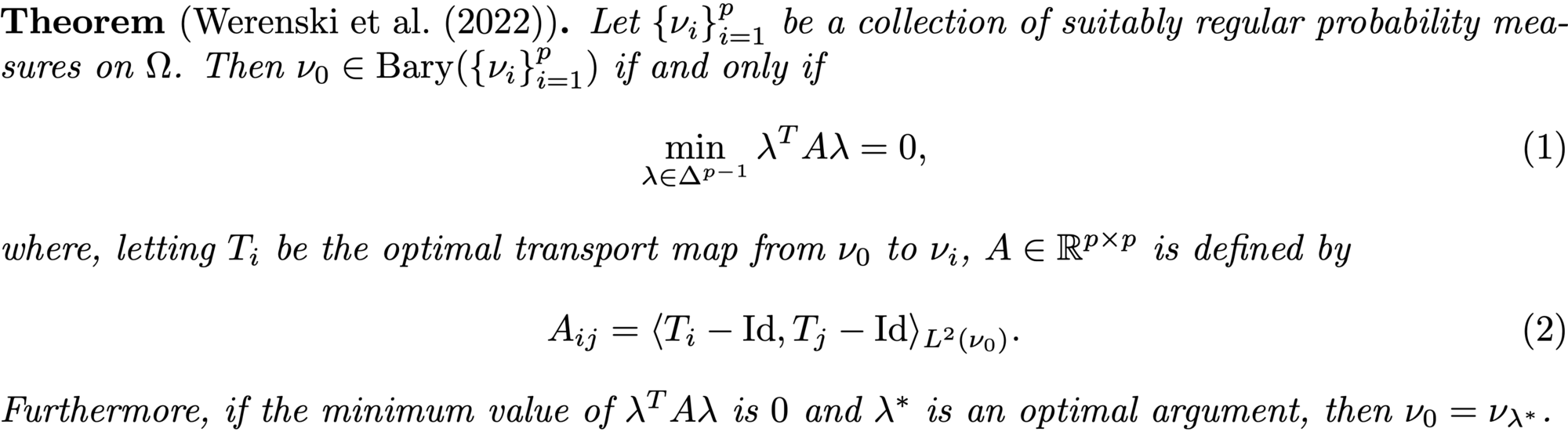
Theorem (Werenski et al. 2022): nu_0 is a barycenter of the references if and only if the minimum over the simplex of lambda^T A lambda is zero, where A_ij is the L2(nu_0) inner product of T_i - Id and T_j - Id; the minimizer recovers the coordinates

Werenski, Matthew, et al. “Measure estimation in the barycentric coding model.” International Conference on Machine Learning. PMLR, 2022.

Ambrosio, Luigi, Nicola Gigli, and Giuseppe Savaré. Gradient flows: in metric spaces and in the space of probability measures. Basel: Birkhäuser Basel, 2005.

Putting it All Together

Summary of Needs

So in short we need:
- To be able to differentiate the variance functional \(J\), in order to identify the direction to walk in when synthesizing a measure
- To be able to approximate the exponential mapping at a measure \(\nu \in \P(X)\) in order to “walk forward” towards the final synthesis measure
- To be able to approximate the inverse of the exponential mapping to lift manifold points into the tangent space, and form the quadratic program which we will solve to analyze measures

Key Idea:

Approximating Geodesic Curves in the \(\W\) geometry

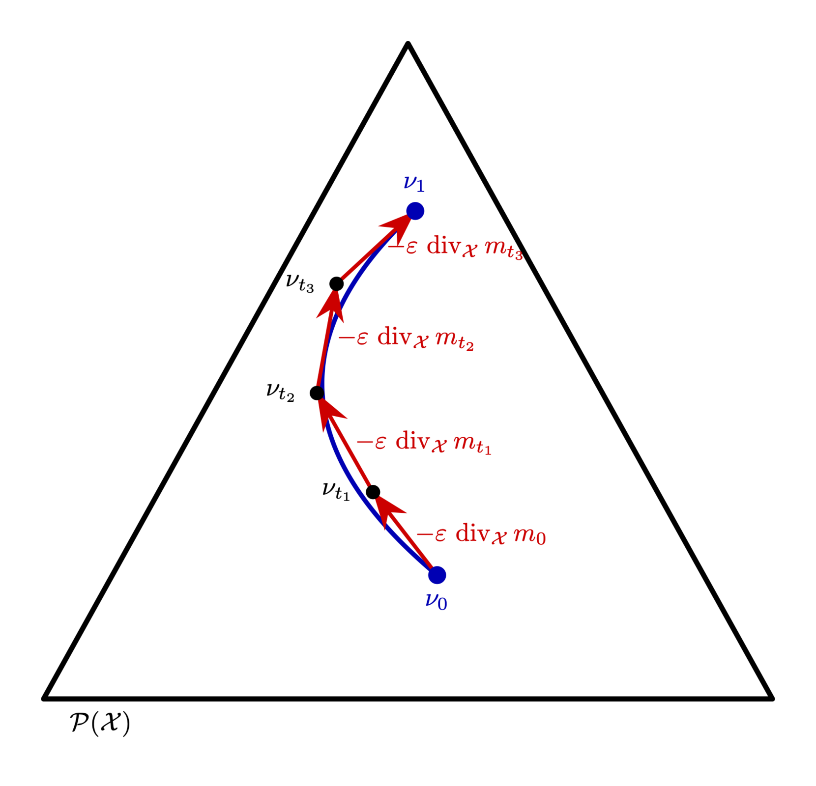
A simplex of measures with a discretized geodesic curve between two of its points

Approximating Geodesic Curves via Chambolle-Pock

One Neat Trick

Erbar et al. (2020) proposed a method for approximating the numerical value of \(\W\) by applying a non-smooth convex optimization algorithm
At a high level: use a weak formulation of the CE, introduce slack variables to decouple variables, minimize the action via Chambolle-Pock

Erbar, Matthias, et al. “Computation of optimal transport on discrete metric measure spaces.” Numerische Mathematik 144.1 (2020): 157–200.

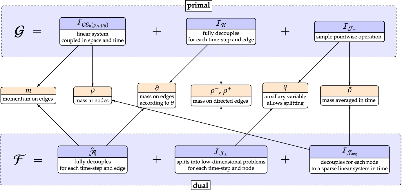
Approximating Geodesic Curves via Chambolle-Pock

It’s simple, really.

Diagram from Erbar et al. (2020) of the constraint sets and proximal maps in their Chambolle-Pock scheme

Erbar, Matthias, et al. “Computation of optimal transport on discrete metric measure spaces.” Numerische Mathematik 144.1 (2020): 157–200.

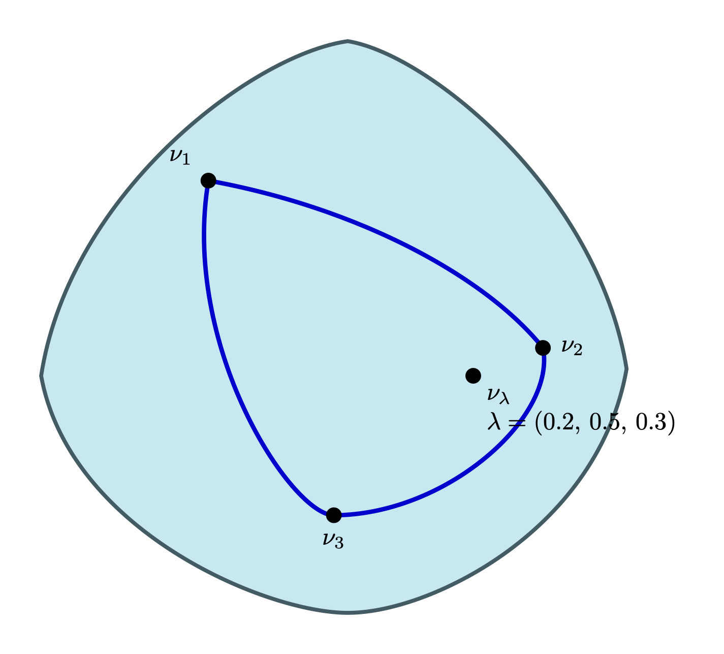
Synthesizing Barycenters of Measures

Key idea: choose the update direction using Riemannian calculus

Geodesics from the current iterate to each reference measure on the manifold

The direction we need to walk in is the direction in the tangent space which most rapidly decreases \(J\)
We can use generic results from Riemannian geometry to differentiate \(J\)

\[ \nabla_{\W} \left\{ \sum_{i=1}^{p} \frac{\lambda_i}{2} \W^2(\nu_i, \nu) \right\} = -\sum_{i=1}^{p} \lambda_i \exp_\nu^{-1}(\nu_i) \]

Synthesizing Barycenters of Measures

Key idea: evolve forward via the continuity equation

In order to update our descent iterates we need to be able to “walk in the direction of steepest descent”, i.e. evaluate the exponential map at least near the current iterate
Our update step will therefore be (for \(0 < t_k \ll 1\))
\[ \nu_{k+1} = \exp_{\nu_k}\left( -t_k \left( \sum_{i=1}^{p} \lambda_i \exp_{\nu_k}^{-1}(\nu_i) \right) \right) \]
Observation: geodesic curves must obey the discretized continuity equation
Idea: use a heuristic update scheme based on the continuity equation near the “launch point” (current iterate)

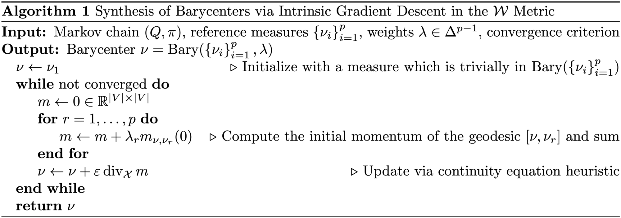
Synthesizing Barycenters of Measures

Update iterates with the continuity equation

If \((\rho, m)\) is a pair satisfying the continuity equation, then we have
\[ \lim_{\varepsilon \to 0} \frac{\rho(t + \varepsilon) - \rho(t)}{\varepsilon} = -\divX(m(t)) \]
So take \(\varepsilon > 0\) to be small, set \(t = 0\), and re-arrange to obtain
\[ \rho(\varepsilon) \approx \rho(0) - \varepsilon \divX m(0) \]
Idea: this update is an approximation of the exponential map near the probability measure \(\rho(0)\)

Synthesizing Barycenters of Measures

An algorithm for synthesis of a barycenter

Algorithm 1: synthesis of barycenters via intrinsic gradient descent in the W metric

Analyzing Barycenters

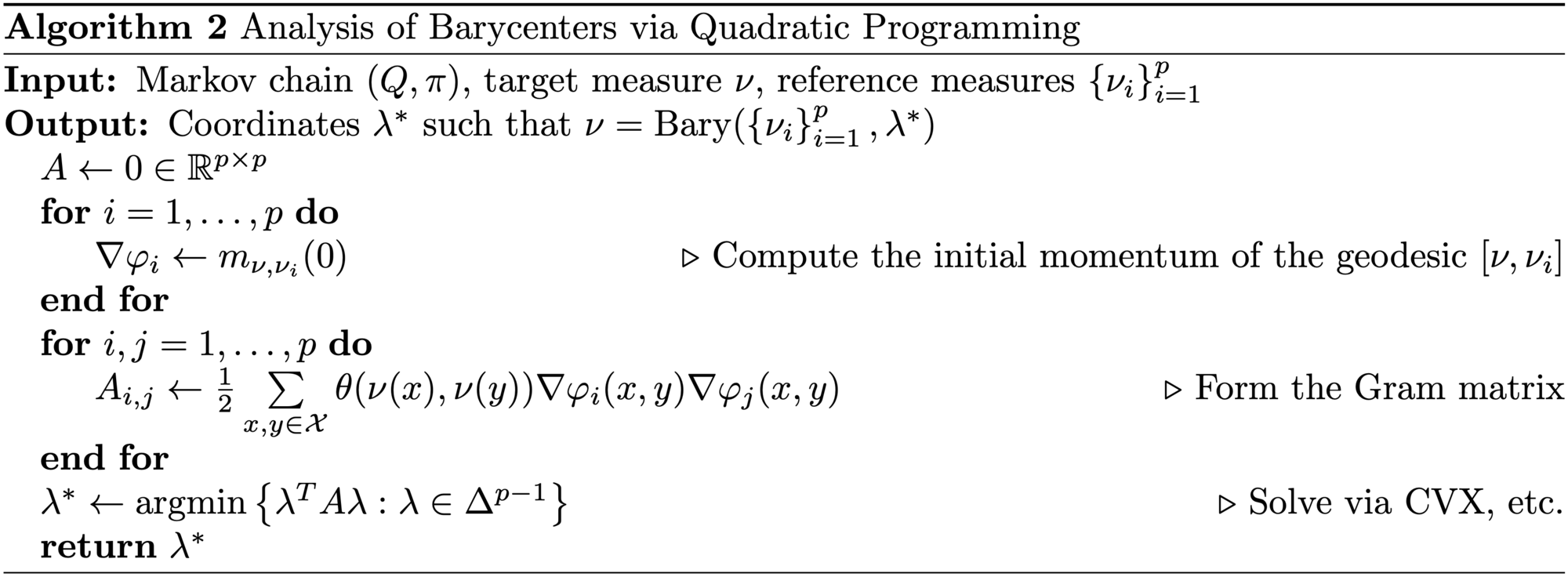
An algorithm for analysis of a measure relative to references

Algorithm 2: analysis of barycenters via quadratic programming

Hyperparameters of the Algorithms

Our algorithms involve 4 hyperparameters:
- \(\delta_g\) — convergence threshold for Chambolle-Pock
- \(N\) — number of steps per geodesic
- \(\delta_b\) — convergence threshold for synthesis gradient descent
- \(\varepsilon\) — step size for gradient descent
Each geodesic is expensive to compute, with complexity scaling quadratically in both \(N\) and \(|V|\)

Numerical Experiments

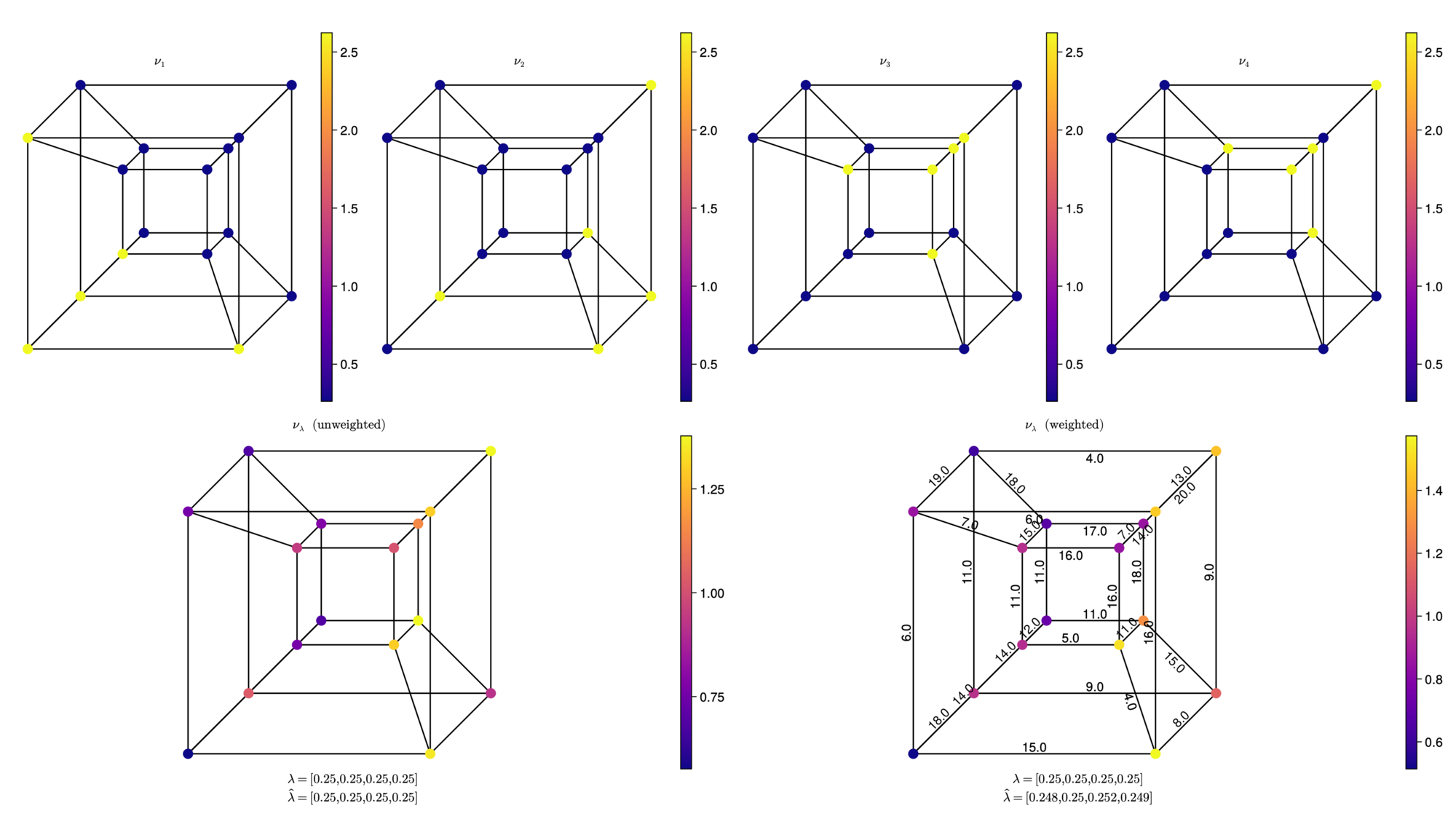
Four reference measures on the hypercube graph and their barycenter, for uniformly and randomly weighted edges

Two Important Questions

Unicity & Consistency of the Implementation

For a fixed family of references \(\Refs = \{\nu_i\}_{i=1}^{p}\), there are two important properties a BCM should have
1. Barycenters should be uniquely specified by their coordinates \(\lambda\)
2. Coordinates recovered via analysis (Alg. 2) of a synthesized measure should be consistent with the coordinates specified when synthesizing; i.e., if \(\nu_\lambda\) is the output of Alg. 1 for inputs \((\lambda, \Refs)\), and \(\hat\lambda\) is the output of Alg. 2 for inputs \((\nu_\lambda, \Refs)\), then we should have that \(\lambda \approx \hat\lambda\)
In numerical simulations, we find both these properties to hold

Descent Initialization

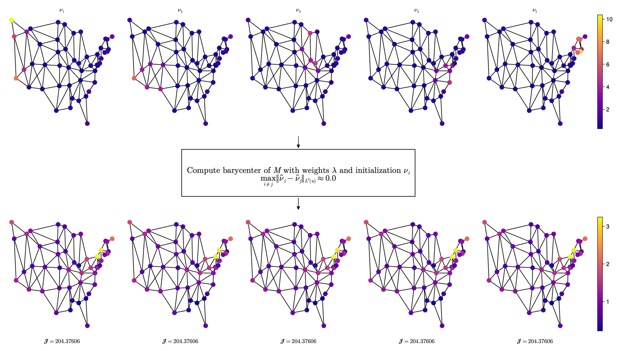
Changing the initialization used for descent doesn’t seem to impact outputs

Barycenters on the US states graph computed from several different initializations; the outputs are visually identical

Coordinate Recovery & Hyperparameters

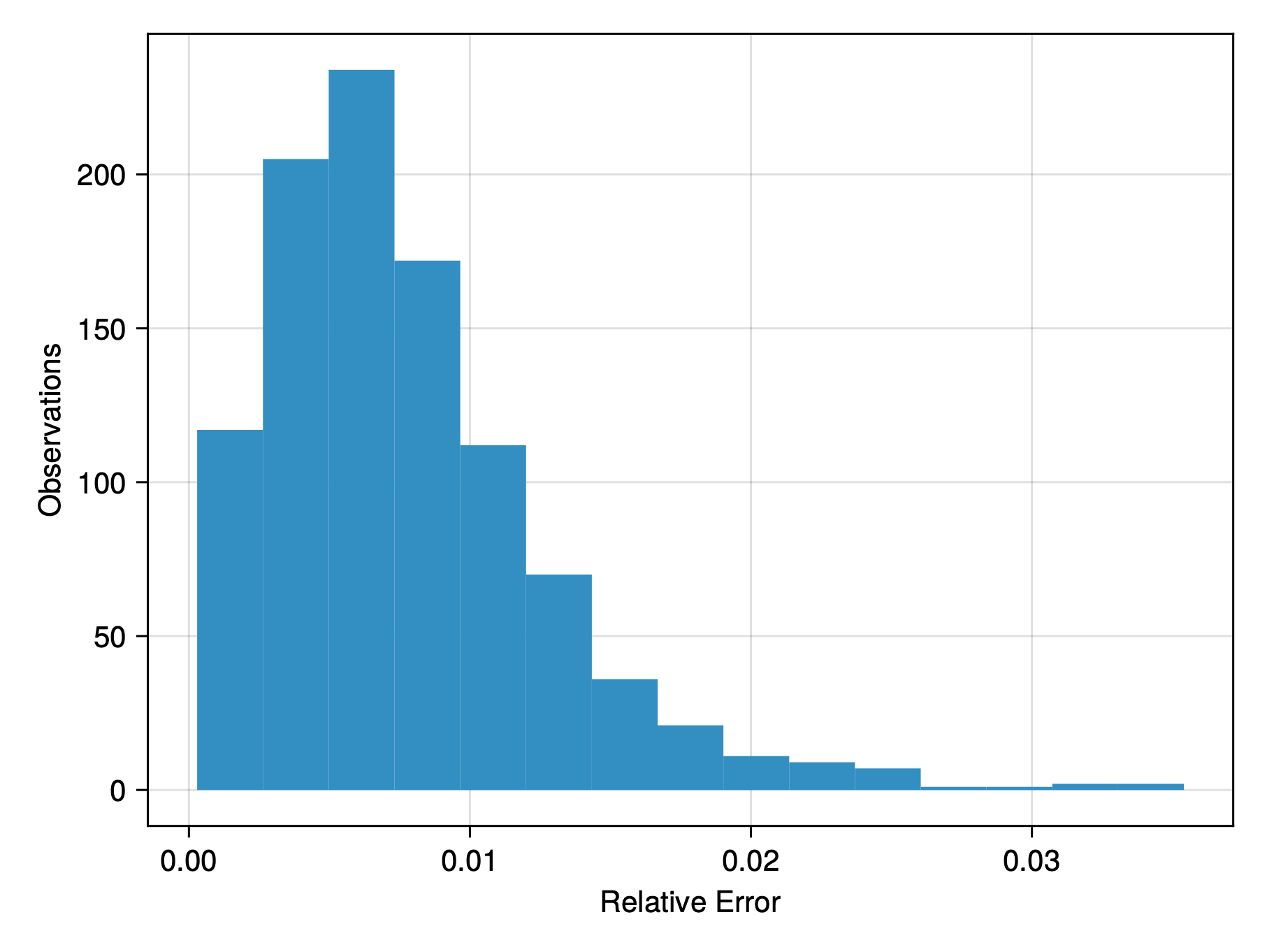
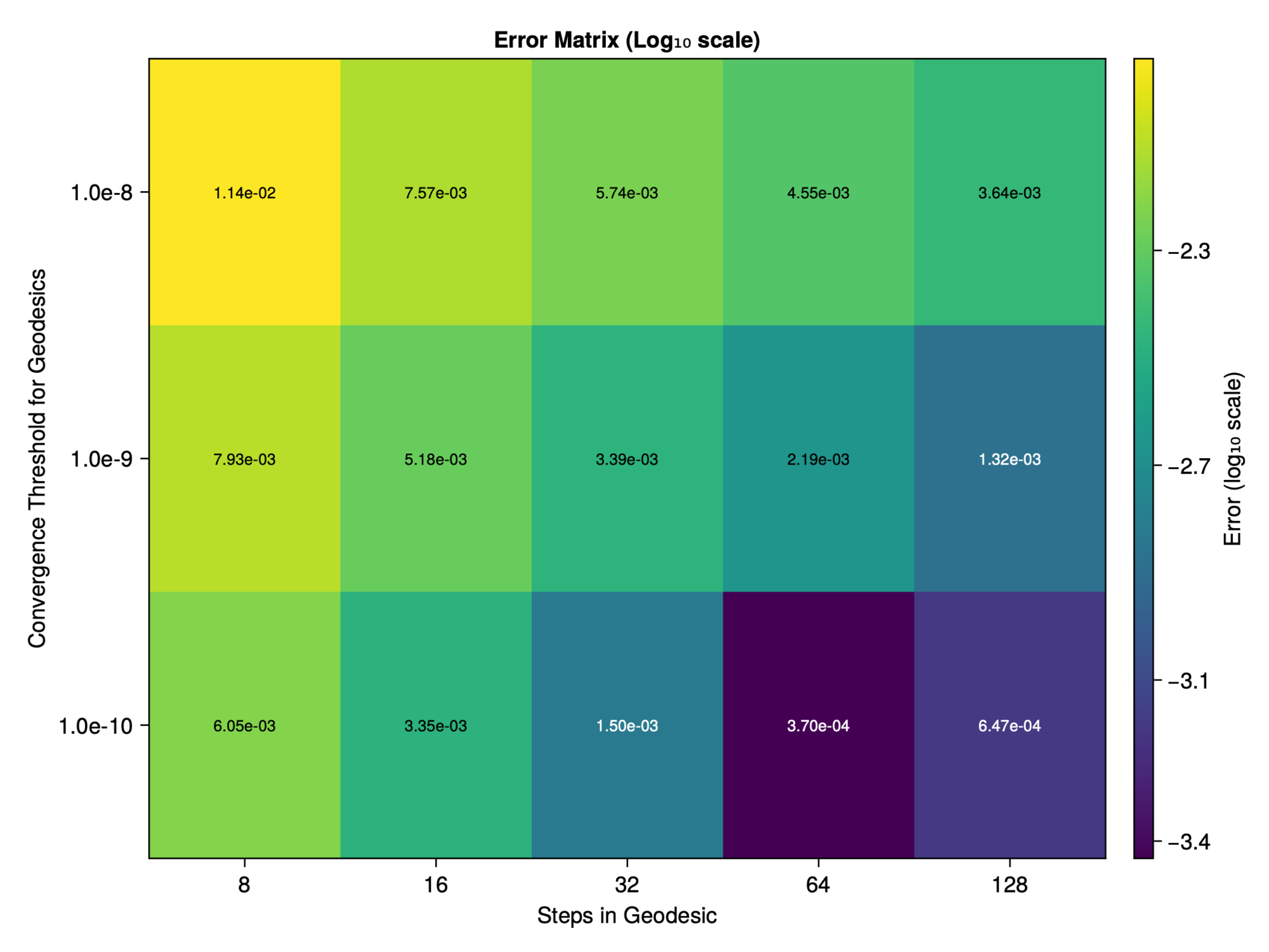
Our synthesis and analysis algorithms are consistent with each other

Histogram of 1000 relative errors in recovered coordinates, concentrated near zero

Heatmap of coordinate recovery error as a function of geodesic convergence threshold and steps per geodesic

Distribution of 1000 observed relative errors in recovery of coordinates from a barycenter synthesized via intrinsic gradient descent for a grid graph on 16 nodes, 3 random measures, a random set of coordinates λ ∈ ∆², with hyperparameters δ_g = 10⁻⁹, N = 10, ε = 0.5, δ_b = 10⁻¹⁰.

Error matrix for coordinate recovery experiment. A graph defined by the 48 contiguous states + D.C. is fixed and three measures ν₁, ν₂, ν₃ are generated randomly, along with randomly chosen coordinates λ. The barycenter ν_λ is computed via intrinsic gradient descent, and then analyzed by solving the associated quadratic program. The relative error of the recovered coordinates is recorded as a function of the convergence threshold for the geodesic computations and the number of steps in each geodesic. Convergence threshold for the barycenters is set to δ_g = 10⁻⁸, and stepsize is taken to be ε = 0.05.

A “Static” Approach to Barycenters of Measures

Entropic Regularization

Popular tool in computational transport: entropic regularization
Main thrust: regularize the Kantorovich problem with an entropy term and apply Sinkhorn’s algorithm to optimize
How it works: fix a regularization parameter \(\varepsilon_{reg} > 0\), encode the graph with a cost matrix \(C\) and solve the regularized K.P.

\[ \OT_{reg}(\mu, \nu) = \inf\left\{ \langle \gamma, C \rangle + \varepsilon_{reg} H(\gamma) : \gamma \in \Pi(\mu, \nu) \right\} \]

\[ H(\gamma) \equiv -\sum_{x,y \in X} \gamma(x,y)\left(\log \gamma(x,y) - 1\right) \]

Comparison with a “Static” Approach To Computing Barycenters

Entropic Transport

Upsides: very fast, can have much better recovery, though not always
Downsides: distance matrices don’t capture all connectivity information, and entropy introduces a bias to the output

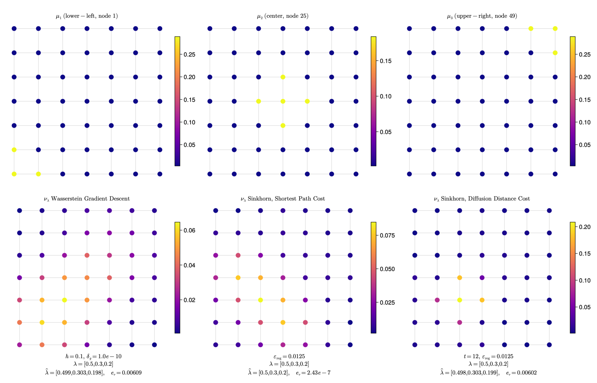
Grid-graph barycenters computed with the dynamic method and with entropic regularization under several cost matrices

Empirical convergence

We can track the norm of the gradient over the course of descent, and we see that it is in line with what we would expect from “standard” gradient descent methods
Possible advancement: use momentum information to accelerate descent? Area of active interest in the Riemannian optimization community

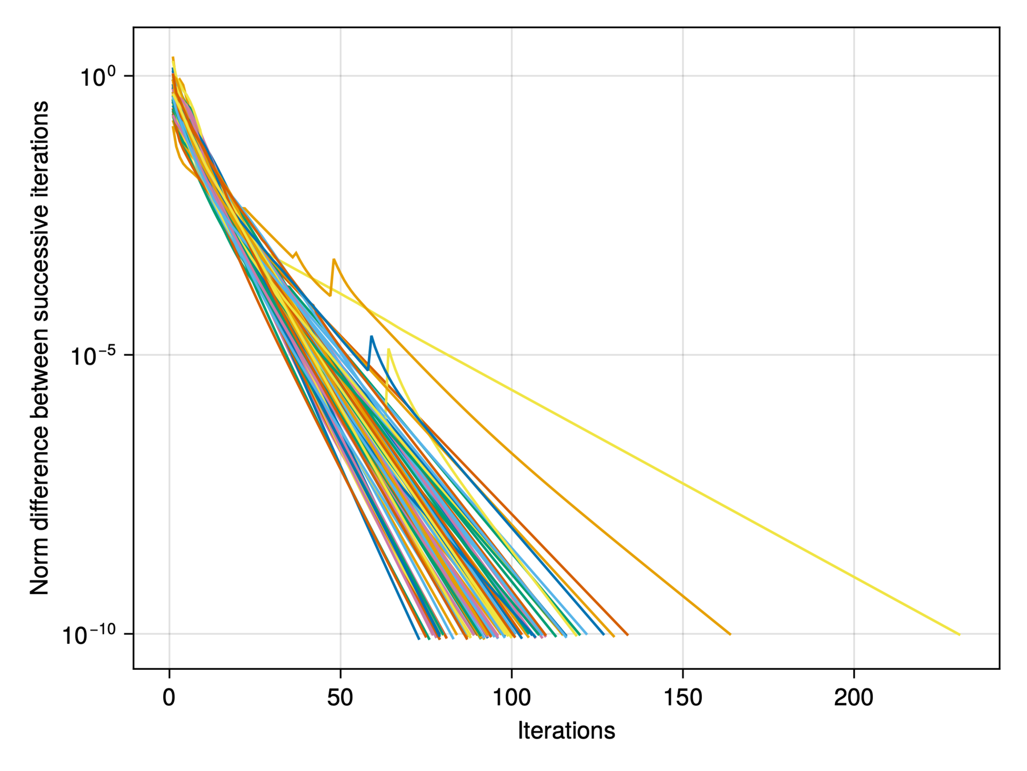
Log-linear plot of the norm difference between successive iterates against iteration count: straight, decreasing lines

Looking Ahead

Future directions and ideas to explore

Key takeaway: we can use the Riemannian geometry, our understanding of the continuity equation, and some non-smooth convex optimization algorithms to synthesize and analyze barycenters of measures on graphs
Building out the theory:
- Make rigorous guarantees about convergence of the descent iterates. The literature in general Riemannian optimization tells us we need more information about the injectivity radius of \((\P(X), \W)\) and some estimate on the eigenvalues of the Riemannian Hessian to identify a region of guaranteed convergence for the synthesis algorithm. The latter could potentially be estimated numerically on a graph-by-graph basis.
- Locality issues: there are graph-connectivity conditions that guarantee the support of the geodesic bridging two measures can be contained to a set \(A \subset V\) — could this kind of a result be extended to the case of a general barycenter?
- Study what happens on the boundary — it can happen that a geodesic connecting two points on the interior of the simplex touches the boundary, but can the conditions under which this occurs be directly characterized, and does it have serious implications for our numerical implementation?

References

My papers:
- G., Huang, and Murphy. “Wasserstein-based identification of metastable states in time series data via change point detection and segment clustering.” arXiv preprint arXiv:2603.01989 (2026).
- G., Murphy. “Static and Dynamic Approaches to Computing Barycenters of Probability Measures on Graphs.” arXiv preprint arXiv:2603.26940 (2026).
My code:
- https://github.com/dcgentile/GraphTransportation.jl
- https://github.com/dcgentile/mfpy
Select references:
- Benamou, Jean-David, and Yann Brenier. “A computational fluid mechanics solution to the Monge-Kantorovich mass transfer problem.” Numerische Mathematik 84.3 (2000): 375–393.
- Agueh, Martial, and Guillaume Carlier. “Barycenters in the Wasserstein space.” SIAM Journal on Mathematical Analysis 43.2 (2011): 904–924.
- Bonneel, Nicolas, Gabriel Peyré, and Marco Cuturi. “Wasserstein barycentric coordinates: histogram regression using optimal transport.” ACM Trans. Graph. 35.4 (2016): 71-1.
- Werenski, Matthew, et al. “Measure estimation in the barycentric coding model.” International Conference on Machine Learning. PMLR, 2022.
- Maas, Jan. “Gradient flows of the entropy for finite Markov chains.” Journal of Functional Analysis 261.8 (2011): 2250–2292.
- Erbar, Matthias, et al. “Computation of optimal transport on discrete metric measure spaces.” Numerische Mathematik 144.1 (2020): 157–200.
- Gangbo, Wilfrid, Wuchen Li, and Chenchen Mou. “Geodesics of minimal length in the set of probability measures on graphs.” ESAIM: Control, Optimisation and Calculus of Variations 25 (2019): 78.
- Afsari, Bijan, Roberto Tron, and René Vidal. “On the convergence of gradient descent for finding the Riemannian center of mass.” SIAM Journal on Control and Optimization 51.3 (2013): 2230–2260.
- Damjanovic, Jovan, James M. Murphy, and Yu-Shan Lin. “Catboss: Cluster analysis of trajectories based on segment splitting.” Journal of Chemical Information and Modeling 61.10 (2021): 5066–5081.
- Ramdas, Aaditya, Nicolás García Trillos, and Marco Cuturi. “On Wasserstein two-sample testing and related families of nonparametric tests.” Entropy 19.2 (2017): 47.

Acknowledgements

Some people and creatures I’d like to thank

Thank you so much for your support and kindness over the years:

My advisor James M. Murphy.

The members of my committee: Kasso Okoudjou, Abiy Tasissa, and Maria Cameron.

My colleagues at Analysis Group: Stefano Parravano, Upamanu Pathare, and Esteban Léon, and at the Naval Research Laboratory: Roger M. Oba, Laurie T. Fialkowski.

The wonderful weirdos of Sarah Lawrence College: Sarah Dennis, Olif Olson, Cole Cuthbert, Brooke Prakash, Isabella Romano, and Hannah Ford, as well as Profs. Mike Siff, Philip Ording, and Melissa Frazier.

The oddballs of Oregon: Thaís De Faria, Daniel Dougherty, Ben McDowell, Annie Price, Jess Lohrman, Adam and Stacy York, Luca Zocchi, Willow Davis, and the greater DWJ Lab family.

The many friends I’ve made at Tufts University: Merek Johnson, David Cohen, Brendan Mallery, Chandler Smith, Martin Buck, and Kecheng Li.

The inimitable Shane Frisco, you are an inspiration.

My family: my mother Linda especially, and also my brother Geof, my uncle Jack, and aunt Jeanne, and my in-laws Jeni, Kevin, Mason, Austin, and Riley Bates, for all their support over the years.

Finally, my amazing wife Dr. Hannah J. Bates, and our two perfect kittens Ezra and Kali, the best cats in this town or any other.